Example: Grover’s Search Algorithm

This example demonstrates an end-to-end quantum computation using the SDK’s DataArray analysis features. It requires Qiskit for circuit construction, which can be installed alongside the SDK:

pip install oqc-qcaas-sdk qiskit

Background

Classical search through N items requires — in the worst case — checking all N of them one at a time. Grover’s algorithm exploits quantum superposition to find a marked item in roughly √N steps instead, a quadratic speedup that is one of the best-proven advantages of quantum computing over classical.

The algorithm works in three stages:

1. Superposition — all qubits are put into an equal mixture of every possible state simultaneously using Hadamard gates (H in the circuit diagram). For 3 qubits this creates a superposition of all 8 states 000 through 111 at once.

2. Oracle — a PhaseOracleGate acts as a “marking” device: it flips the quantum phase of one specific target state without disturbing the others or measuring anything. The phase flip is invisible to a direct measurement but influences subsequent interference.

3. Diffusion (Grover operator) — the grover_operator amplifies the probability of the marked state and suppresses all others. After one iteration the marked state is significantly more likely to be the outcome when the qubits are measured.

The scenario

The example runs eight separate Grover circuits in parallel, one per possible 3-bit answer ("000" through "111"). Each circuit is tuned to amplify exactly one target bitstring. All eight are submitted as a single CompositeJob and polled concurrently.

When the results come back, a single call converts all eight results into one labelled 2-D DataArray:

• Rows — one per Grover circuit (i.e. one per target bitstring)

• Columns — one per observed bitstring outcome

We expect the DataArray to be peaked on the diagonal: the circuit targeting "000" should measure mostly "000", the one targeting "001" mostly "001", and so on. Normalising by total shots converts raw counts to probability distributions, making the diagonal structure visually clear.

Building the circuits

The Qiskit helper converts a target bitstring into an OpenQASM 2 string that you can execute with the SDK.

from qiskit.circuit.library import PhaseOracleGate, grover_operator
from qiskit.circuit import QuantumCircuit
from qiskit import qasm2


def bitstring_to_expression(bitstring: str) -> str:
    """Convert a bitstring to a boolean expression for the phase oracle.

    Each character position becomes a logical variable (a, b, c, ...).
    A '1' bit contributes the variable directly; a '0' bit contributes its
    negation.  The expression uniquely identifies the target state.

    Examples:
        "011" → "~a & b & c"   (qubit 0 must be 0, qubits 1 and 2 must be 1)
        "101" → "a & ~b & c"
    """
    var_names = [chr(ord("a") + i) for i in range(len(bitstring))]
    terms = [v if b == "1" else f"~{v}" for b, v in zip(bitstring, var_names)]
    return " & ".join(terms)


def build_circuit(marked_state: str) -> str:
    """Build a Grover search circuit targeting *marked_state*, as OpenQASM 2.

    The circuit applies one Grover iteration:

    1. Hadamard gates create equal superposition of all 2**n states.
    2. A phase oracle marks the target state.
    3. The Grover diffusion operator amplifies the marked state's probability.
    4. All qubits are measured into a classical register ``c``.
    """
    oracle = PhaseOracleGate(bitstring_to_expression(marked_state))
    grover_op = grover_operator(oracle)

    n = len(marked_state)
    qc = QuantumCircuit(n, n)
    qc.h(range(n))           # uniform superposition
    qc.compose(grover_op, inplace=True)
    qc.measure(range(n), range(n))

    return qasm2.dumps(qc)

Executing with CompositeJob

For 3 qubits there are 2³ = 8 possible bitstrings, so we build 8 circuits and submit them all at once. CompositeJob handles the batch submission and concurrent polling automatically.

import asyncio
from oqc_qcaas_sdk import OqcSdk

QPU_ID = "qpu:uk:2:d865b5a184"  # Simulator

async def run_all_marked_states(nqubits: int, url: str, token: str):
    async with OqcSdk(url=url, authentication_token=token) as client:
        # One circuit per possible bitstring: "000", "001", ..., "111"
        programs = [
            build_circuit(format(i, f"0{nqubits}b"))
            for i in range(2**nqubits)
        ]
        cjob = client.create_job(program=programs, qpu_id=QPU_ID)
        return await cjob.execute(timeout_s=60)

outputs = asyncio.run(run_all_marked_states(3, url=URL, token=TOKEN))

The returned outputs is a JobOutputProxy holding one JobResult per circuit.

Analysing the results

Because to_counts_dataarray() aggregates every result in a proxy into a single DataArray, the entire analysis is a one-liner:

import scipp as sc

da = outputs.to_counts_dataarray(creg="c")
# da.shape == (8, 8)
# da["result", bits("000")] → counts from the circuit targeting "000"
# da["result", bits("111")] → counts from the circuit targeting "111"

The raw counts DataArray looks like this (truncated for clarity):

<scipp.DataArray>
Dimensions: Sizes[result:8, bit:8]
Coordinates:
* result    int64  [dimensionless]  [0, 1, ..., 7]
* bit       int64  [dimensionless]  [0, 1, ..., 7]
  bitstring str    [dimensionless]  ["000", "001", ..., "111"]
Data:
  int64  [dimensionless]  [[8, 3, 2, ...], [2, 9, 1, ...], ...]

A quick plot of the raw counts reveals the diagonal structure already:

da.plot()

To make the diagonal cleaner and comparable across runs with different shot counts, normalise each row by dividing by the total counts in that row:

da_norm = da / sc.sum(da, dim="bit")
da_norm.plot()

Each row of da_norm is now a probability distribution over bitstrings. A Grover circuit working correctly will put nearly all its probability mass on the diagonal entry — the one bitstring it was designed to find.

What a successful result looks like

After normalisation, the diagonal entry for each row should be significantly larger than all off-diagonal entries. For a 3-qubit Grover search with one iteration, theory predicts roughly 78% probability on the marked state (leaving ~3% each on the 7 remaining states). Shot noise and real QPU imperfections will smear this, but the diagonal structure should remain visible.

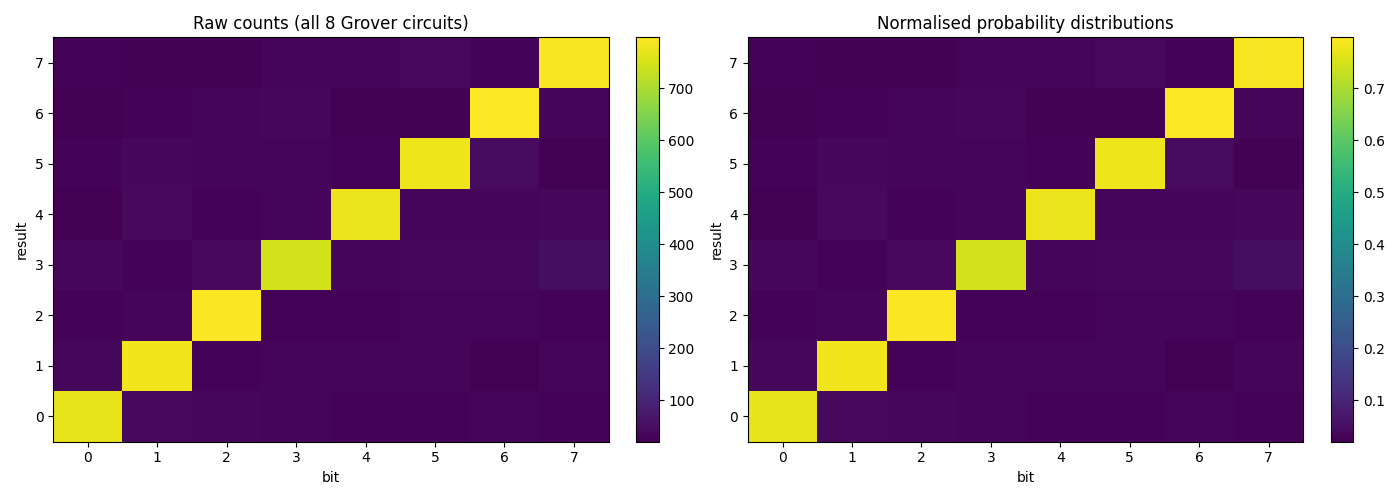
Output of the two plot() calls above — raw counts (left) and per-row normalised probabilities (right). The diagonal structure confirms each circuit is finding its target bitstring.

You can extract the diagonal probabilities directly:

import numpy as np

# Probability of measuring the marked state for each circuit
diag_probs = [float(da_norm["result", i]["bit", i].value) for i in range(8)]
print(diag_probs)  # e.g. [0.77, 0.75, 0.79, ...]

Wildcard filtering

The like() method lets you focus on a subset of bitstrings without slicing indices manually. For example, to see only the counts for bitstrings where the most-significant bit (leftmost in OQC’s big-endian notation) is 1:

high = outputs.like("1**", creg="c")
# high.shape == (8, 4)  — all 8 runs, only bitstrings 4..7